
Getting started with Advanced HPO Algorithms
Loading libraries
# Basic utils for folder manipulations etc
import time
import multiprocessing # to count the number of CPUs available

# External tools to load and process data
import numpy as np
import pandas as pd

# MXNet (NeuralNets)
import mxnet as mx
from mxnet import gluon, autograd
from mxnet.gluon import nn

# AutoGluon and HPO tools
import autogluon.core as ag
from autogluon.mxnet.utils import load_and_split_openml_data
Check the version of MxNet, you should be fine with version >= 1.5
mx.__version__
'1.7.0'
You can also check the version of AutoGluon and the specific commit and check that it matches what you want.
import autogluon.core.version
ag.version.__version__
'0.0.15b20201023'
Hyperparameter Optimization of a 2-layer MLP
Setting up the context
Here we declare a few “environment variables” setting the context for what we’re doing
OPENML_TASK_ID = 6                # describes the problem we will tackle
RATIO_TRAIN_VALID = 0.33          # split of the training data used for validation
RESOURCE_ATTR_NAME = 'epoch'      # how do we measure resources   (will become clearer further)
REWARD_ATTR_NAME = 'objective'    # how do we measure performance (will become clearer further)

NUM_CPUS = multiprocessing.cpu_count()
Preparing the data
We will use a multi-way classification task from OpenML. Data preparation includes:
Missing values are imputed, using the ‘mean’ strategy of
sklearn.impute.SimpleImputerSplit training set into training and validation
Standardize inputs to mean 0, variance 1
X_train, X_valid, y_train, y_valid, n_classes = load_and_split_openml_data(
    OPENML_TASK_ID, RATIO_TRAIN_VALID, download_from_openml=False)
n_classes
100%|██████████| 704/704 [00:00<00:00, 35501.36KB/s]
100%|██████████| 2521/2521 [00:00<00:00, 37980.07KB/s]
3KB [00:00, 2397.20KB/s]
8KB [00:00, 5451.57KB/s]
15KB [00:00, 11109.76KB/s]
2998KB [00:00, 18504.25KB/s]
881KB [00:00, 50787.29KB/s]
3KB [00:00, 2444.23KB/s]
26
The problem has 26 classes.
Declaring a model specifying a hyperparameter space with AutoGluon
Two layer MLP where we optimize over:
the number of units on the first layer
the number of units on the second layer
the dropout rate after each layer
the learning rate
the scaling
the
@ag.argsdecorator allows us to specify the space we will optimize over, this matches the ConfigSpace syntax
The body of the function run_mlp_openml is pretty simple:
it reads the hyperparameters given via the decorator
it defines a 2 layer MLP with dropout
it declares a trainer with the ‘adam’ loss function and a provided learning rate
it trains the NN with a number of epochs (most of that is boilerplate code from
mxnet)the
reporterat the end is used to keep track of training history in the hyperparameter optimization
Note: The number of epochs and the hyperparameter space are reduced to make for a shorter experiment
@ag.args(n_units_1=ag.space.Int(lower=16, upper=128),
         n_units_2=ag.space.Int(lower=16, upper=128),
         dropout_1=ag.space.Real(lower=0, upper=.75),
         dropout_2=ag.space.Real(lower=0, upper=.75),
         learning_rate=ag.space.Real(lower=1e-6, upper=1, log=True),
         batch_size=ag.space.Int(lower=8, upper=128),
         scale_1=ag.space.Real(lower=0.001, upper=10, log=True),
         scale_2=ag.space.Real(lower=0.001, upper=10, log=True),
         epochs=9)
def run_mlp_openml(args, reporter, **kwargs):
    # Time stamp for elapsed_time
    ts_start = time.time()
    # Unwrap hyperparameters
    n_units_1 = args.n_units_1
    n_units_2 = args.n_units_2
    dropout_1 = args.dropout_1
    dropout_2 = args.dropout_2
    scale_1 = args.scale_1
    scale_2 = args.scale_2
    batch_size = args.batch_size
    learning_rate = args.learning_rate

    ctx = mx.cpu()
    net = nn.Sequential()
    with net.name_scope():
        # Layer 1
        net.add(nn.Dense(n_units_1, activation='relu',
                         weight_initializer=mx.initializer.Uniform(scale=scale_1)))
        # Dropout
        net.add(gluon.nn.Dropout(dropout_1))
        # Layer 2
        net.add(nn.Dense(n_units_2, activation='relu',
                         weight_initializer=mx.initializer.Uniform(scale=scale_2)))
        # Dropout
        net.add(gluon.nn.Dropout(dropout_2))
        # Output
        net.add(nn.Dense(n_classes))
    net.initialize(ctx=ctx)

    trainer = gluon.Trainer(net.collect_params(), 'adam',
                            {'learning_rate': learning_rate})

    for epoch in range(args.epochs):
        ts_epoch = time.time()

        train_iter = mx.io.NDArrayIter(
                        data={'data': X_train},
                        label={'label': y_train},
                        batch_size=batch_size,
                        shuffle=True)
        valid_iter = mx.io.NDArrayIter(
                        data={'data': X_valid},
                        label={'label': y_valid},
                        batch_size=batch_size,
                        shuffle=False)

        metric = mx.metric.Accuracy()
        loss = gluon.loss.SoftmaxCrossEntropyLoss()

        for batch in train_iter:
            data = batch.data[0].as_in_context(ctx)
            label = batch.label[0].as_in_context(ctx)
            with autograd.record():
                output = net(data)
                L = loss(output, label)
            L.backward()
            trainer.step(data.shape[0])
            metric.update([label], [output])

        name, train_acc = metric.get()

        metric = mx.metric.Accuracy()
        for batch in valid_iter:
            data = batch.data[0].as_in_context(ctx)
            label = batch.label[0].as_in_context(ctx)
            output = net(data)
            metric.update([label], [output])

        name, val_acc = metric.get()

        print('Epoch %d ; Time: %f ; Training: %s=%f ; Validation: %s=%f' % (
            epoch + 1, time.time() - ts_start, name, train_acc, name, val_acc))

        ts_now = time.time()
        eval_time = ts_now - ts_epoch
        elapsed_time = ts_now - ts_start

        # The resource reported back (as 'epoch') is the number of epochs
        # done, starting at 1
        reporter(
            epoch=epoch + 1,
            objective=float(val_acc),
            eval_time=eval_time,
            time_step=ts_now,
            elapsed_time=elapsed_time)
Note: The annotation epochs=9 specifies the maximum number of
epochs for training. It becomes available as args.epochs.
Importantly, it is also processed by HyperbandScheduler below in
order to set its max_t attribute.
Recommendation: Whenever writing training code to be passed as
train_fn to a scheduler, if this training code reports a resource
(or time) attribute, the corresponding maximum resource value should be
included in train_fn.args:
If the resource attribute (
time_attrof scheduler) intrain_fnisepoch, make sure to includeepochs=XYZin the annotation. This allows the scheduler to readmax_tfromtrain_fn.args.epochs. This case corresponds to our example here.If the resource attribute is something else than
epoch, you can also include the annotationmax_t=XYZ, which allows the scheduler to readmax_tfromtrain_fn.args.max_t.
Annotating the training function by the correct value for max_t
simplifies scheduler creation (since max_t does not have to be
passed), and avoids inconsistencies between train_fn and the
scheduler.
Running the Hyperparameter Optimization
You can use the following schedulers:
FIFO (
fifo)Hyperband (either the stopping (
hbs) or promotion (hbp) variant)
And the following searchers:
Random search (
random)Gaussian process based Bayesian optimization (
bayesopt)SkOpt Bayesian optimization (
skopt; only with FIFO scheduler)
Note that the method known as (asynchronous) Hyperband is using random
search. Combining Hyperband scheduling with the bayesopt searcher
uses a novel method called asynchronous BOHB.
Pick the combination you’re interested in (doing the full experiment
takes around 120 seconds, see the time_out parameter), running
everything with multiple runs can take a fair bit of time. In real life,
you will want to choose a larger time_out in order to obtain good
performance.
SCHEDULER = "hbs"
SEARCHER = "bayesopt"
def compute_error(df):
    return 1.0 - df["objective"]

def compute_runtime(df, start_timestamp):
        return df["time_step"] - start_timestamp

def process_training_history(task_dicts, start_timestamp,
                             runtime_fn=compute_runtime,
                             error_fn=compute_error):
    task_dfs = []
    for task_id in task_dicts:
        task_df = pd.DataFrame(task_dicts[task_id])
        task_df = task_df.assign(task_id=task_id,
                                 runtime=runtime_fn(task_df, start_timestamp),
                                 error=error_fn(task_df),
                                 target_epoch=task_df["epoch"].iloc[-1])
        task_dfs.append(task_df)

    result = pd.concat(task_dfs, axis="index", ignore_index=True, sort=True)
    # re-order by runtime
    result = result.sort_values(by="runtime")
    # calculate incumbent best -- the cumulative minimum of the error.
    result = result.assign(best=result["error"].cummin())
    return result

resources = dict(num_cpus=NUM_CPUS, num_gpus=0)
search_options = {
    'num_init_random': 2,
    'debug_log': True}
if SCHEDULER == 'fifo':
    myscheduler = ag.scheduler.FIFOScheduler(
        run_mlp_openml,
        resource=resources,
        searcher=SEARCHER,
        search_options=search_options,
        time_out=120,
        time_attr=RESOURCE_ATTR_NAME,
        reward_attr=REWARD_ATTR_NAME)

else:
    # This setup uses rung levels at 1, 3, 9 epochs. We just use a single
    # bracket, so this is in fact successive halving (Hyperband would use
    # more than 1 bracket).
    # Also note that since we do not use the max_t argument of
    # HyperbandScheduler, this value is obtained from train_fn.args.epochs.
    sch_type = 'stopping' if SCHEDULER == 'hbs' else 'promotion'
    myscheduler = ag.scheduler.HyperbandScheduler(
        run_mlp_openml,
        resource=resources,
        searcher=SEARCHER,
        search_options=search_options,
        time_out=120,
        time_attr=RESOURCE_ATTR_NAME,
        reward_attr=REWARD_ATTR_NAME,
        type=sch_type,
        grace_period=1,
        reduction_factor=3,
        brackets=1)

# run tasks
myscheduler.run()
myscheduler.join_jobs()

results_df = process_training_history(
                myscheduler.training_history.copy(),
                start_timestamp=myscheduler._start_time)
/var/lib/jenkins/miniconda3/envs/autogluon_docs/lib/python3.7/site-packages/distributed/worker.py:3382: UserWarning: Large object of size 1.30 MB detected in task graph:
  (<function run_mlp_openml at 0x7f0c9dfd9c20>, {'ar ... sReporter}, [])
Consider scattering large objects ahead of time
with client.scatter to reduce scheduler burden and
keep data on workers

    future = client.submit(func, big_data)    # bad

    big_future = client.scatter(big_data)     # good
    future = client.submit(func, big_future)  # good
  % (format_bytes(len(b)), s)
Epoch 1 ; Time: 0.483396 ; Training: accuracy=0.260079 ; Validation: accuracy=0.531250
Epoch 2 ; Time: 1.030503 ; Training: accuracy=0.496365 ; Validation: accuracy=0.655247
Epoch 3 ; Time: 1.452055 ; Training: accuracy=0.559650 ; Validation: accuracy=0.694686
Epoch 4 ; Time: 1.872615 ; Training: accuracy=0.588896 ; Validation: accuracy=0.711063
Epoch 5 ; Time: 2.296367 ; Training: accuracy=0.609385 ; Validation: accuracy=0.726939
Epoch 6 ; Time: 2.717657 ; Training: accuracy=0.628139 ; Validation: accuracy=0.745321
Epoch 7 ; Time: 3.140399 ; Training: accuracy=0.641193 ; Validation: accuracy=0.750501
Epoch 8 ; Time: 3.560328 ; Training: accuracy=0.653751 ; Validation: accuracy=0.763202
Epoch 9 ; Time: 3.992006 ; Training: accuracy=0.665482 ; Validation: accuracy=0.766043
Epoch 1 ; Time: 1.905188 ; Training: accuracy=0.053355 ; Validation: accuracy=0.045042
Epoch 1 ; Time: 0.461632 ; Training: accuracy=0.431786 ; Validation: accuracy=0.519320
Epoch 2 ; Time: 0.877436 ; Training: accuracy=0.482336 ; Validation: accuracy=0.555296
Epoch 3 ; Time: 1.303985 ; Training: accuracy=0.501696 ; Validation: accuracy=0.525483
Epoch 1 ; Time: 0.367958 ; Training: accuracy=0.174107 ; Validation: accuracy=0.393098
Epoch 1 ; Time: 0.291390 ; Training: accuracy=0.044229 ; Validation: accuracy=0.057209
Epoch 1 ; Time: 0.385228 ; Training: accuracy=0.399736 ; Validation: accuracy=0.654512
Epoch 2 ; Time: 0.741803 ; Training: accuracy=0.578782 ; Validation: accuracy=0.716783
Epoch 3 ; Time: 1.095011 ; Training: accuracy=0.627117 ; Validation: accuracy=0.770563
Epoch 4 ; Time: 1.448431 ; Training: accuracy=0.656201 ; Validation: accuracy=0.765734
Epoch 5 ; Time: 1.798785 ; Training: accuracy=0.676361 ; Validation: accuracy=0.784549
Epoch 6 ; Time: 2.149667 ; Training: accuracy=0.682062 ; Validation: accuracy=0.795205
Epoch 7 ; Time: 2.500064 ; Training: accuracy=0.688920 ; Validation: accuracy=0.805028
Epoch 8 ; Time: 2.851642 ; Training: accuracy=0.703379 ; Validation: accuracy=0.820180
Epoch 9 ; Time: 3.182056 ; Training: accuracy=0.704288 ; Validation: accuracy=0.815351
Epoch 1 ; Time: 0.522432 ; Training: accuracy=0.039245 ; Validation: accuracy=0.039813
Epoch 1 ; Time: 1.601753 ; Training: accuracy=0.048176 ; Validation: accuracy=0.113636
Epoch 1 ; Time: 0.361345 ; Training: accuracy=0.402804 ; Validation: accuracy=0.673761
Epoch 2 ; Time: 0.713826 ; Training: accuracy=0.619794 ; Validation: accuracy=0.756069
Epoch 3 ; Time: 1.051737 ; Training: accuracy=0.671588 ; Validation: accuracy=0.784835
Epoch 4 ; Time: 1.384798 ; Training: accuracy=0.704990 ; Validation: accuracy=0.801796
Epoch 5 ; Time: 1.715117 ; Training: accuracy=0.713155 ; Validation: accuracy=0.813768
Epoch 6 ; Time: 2.045310 ; Training: accuracy=0.720825 ; Validation: accuracy=0.819255
Epoch 7 ; Time: 2.374821 ; Training: accuracy=0.731794 ; Validation: accuracy=0.820253
Epoch 8 ; Time: 2.684129 ; Training: accuracy=0.739464 ; Validation: accuracy=0.830063
Epoch 9 ; Time: 2.980757 ; Training: accuracy=0.738227 ; Validation: accuracy=0.837047
Epoch 1 ; Time: 0.292695 ; Training: accuracy=0.040543 ; Validation: accuracy=0.036403
Epoch 1 ; Time: 0.576766 ; Training: accuracy=0.648760 ; Validation: accuracy=0.787879
Epoch 2 ; Time: 1.127519 ; Training: accuracy=0.817851 ; Validation: accuracy=0.854377
Epoch 3 ; Time: 1.637516 ; Training: accuracy=0.857686 ; Validation: accuracy=0.879293
Epoch 4 ; Time: 2.136355 ; Training: accuracy=0.878595 ; Validation: accuracy=0.892424
Epoch 5 ; Time: 2.635149 ; Training: accuracy=0.893719 ; Validation: accuracy=0.901515
Epoch 6 ; Time: 3.138106 ; Training: accuracy=0.910000 ; Validation: accuracy=0.912795
Epoch 7 ; Time: 3.639281 ; Training: accuracy=0.912562 ; Validation: accuracy=0.922391
Epoch 8 ; Time: 4.143319 ; Training: accuracy=0.920909 ; Validation: accuracy=0.917172
Epoch 9 ; Time: 4.642261 ; Training: accuracy=0.925455 ; Validation: accuracy=0.917845
Epoch 1 ; Time: 0.320751 ; Training: accuracy=0.533680 ; Validation: accuracy=0.749124
Epoch 2 ; Time: 0.605193 ; Training: accuracy=0.782957 ; Validation: accuracy=0.808173
Epoch 3 ; Time: 0.882367 ; Training: accuracy=0.843045 ; Validation: accuracy=0.867056
Epoch 4 ; Time: 1.161692 ; Training: accuracy=0.874204 ; Validation: accuracy=0.870892
Epoch 5 ; Time: 1.411325 ; Training: accuracy=0.895529 ; Validation: accuracy=0.903086
Epoch 6 ; Time: 1.682578 ; Training: accuracy=0.911067 ; Validation: accuracy=0.907590
Epoch 7 ; Time: 1.936404 ; Training: accuracy=0.924043 ; Validation: accuracy=0.914929
Epoch 8 ; Time: 2.196580 ; Training: accuracy=0.933466 ; Validation: accuracy=0.921935
Epoch 9 ; Time: 2.448288 ; Training: accuracy=0.932308 ; Validation: accuracy=0.919433
Epoch 1 ; Time: 0.301587 ; Training: accuracy=0.392863 ; Validation: accuracy=0.664436
Epoch 2 ; Time: 0.550983 ; Training: accuracy=0.568223 ; Validation: accuracy=0.718970
Epoch 3 ; Time: 0.819783 ; Training: accuracy=0.611856 ; Validation: accuracy=0.750585
Epoch 1 ; Time: 3.768589 ; Training: accuracy=0.622099 ; Validation: accuracy=0.738560
Epoch 2 ; Time: 7.421964 ; Training: accuracy=0.779261 ; Validation: accuracy=0.790040
Epoch 3 ; Time: 10.716829 ; Training: accuracy=0.811257 ; Validation: accuracy=0.818136
Epoch 4 ; Time: 13.979789 ; Training: accuracy=0.836704 ; Validation: accuracy=0.825202
Epoch 5 ; Time: 17.438679 ; Training: accuracy=0.846651 ; Validation: accuracy=0.838829
Epoch 6 ; Time: 20.701848 ; Training: accuracy=0.859334 ; Validation: accuracy=0.853634
Epoch 7 ; Time: 23.978994 ; Training: accuracy=0.872430 ; Validation: accuracy=0.865242
Epoch 8 ; Time: 27.493685 ; Training: accuracy=0.881631 ; Validation: accuracy=0.870794
Epoch 9 ; Time: 30.791887 ; Training: accuracy=0.886936 ; Validation: accuracy=0.861541
Epoch 1 ; Time: 2.384123 ; Training: accuracy=0.246270 ; Validation: accuracy=0.583908
Epoch 1 ; Time: 0.472102 ; Training: accuracy=0.486028 ; Validation: accuracy=0.705154
Epoch 2 ; Time: 0.864719 ; Training: accuracy=0.672867 ; Validation: accuracy=0.797523
Epoch 3 ; Time: 1.248857 ; Training: accuracy=0.733962 ; Validation: accuracy=0.820783
Epoch 4 ; Time: 1.632525 ; Training: accuracy=0.768022 ; Validation: accuracy=0.849398
Epoch 5 ; Time: 2.014390 ; Training: accuracy=0.794478 ; Validation: accuracy=0.863621
Epoch 6 ; Time: 2.409124 ; Training: accuracy=0.819775 ; Validation: accuracy=0.882530
Epoch 7 ; Time: 2.836029 ; Training: accuracy=0.833664 ; Validation: accuracy=0.891064
Epoch 8 ; Time: 3.217961 ; Training: accuracy=0.840112 ; Validation: accuracy=0.895917
Epoch 9 ; Time: 3.605930 ; Training: accuracy=0.852679 ; Validation: accuracy=0.896586
Epoch 1 ; Time: 0.620130 ; Training: accuracy=0.590909 ; Validation: accuracy=0.763361
Epoch 2 ; Time: 1.243190 ; Training: accuracy=0.803306 ; Validation: accuracy=0.848403
Epoch 3 ; Time: 1.858045 ; Training: accuracy=0.863140 ; Validation: accuracy=0.874118
Epoch 4 ; Time: 2.491164 ; Training: accuracy=0.890992 ; Validation: accuracy=0.876471
Epoch 5 ; Time: 3.062593 ; Training: accuracy=0.906033 ; Validation: accuracy=0.878319
Epoch 6 ; Time: 3.641355 ; Training: accuracy=0.924628 ; Validation: accuracy=0.921345
Epoch 7 ; Time: 4.225958 ; Training: accuracy=0.930909 ; Validation: accuracy=0.922857
Epoch 8 ; Time: 4.798274 ; Training: accuracy=0.935537 ; Validation: accuracy=0.930084
Epoch 9 ; Time: 5.367144 ; Training: accuracy=0.940000 ; Validation: accuracy=0.917311
Epoch 1 ; Time: 1.036110 ; Training: accuracy=0.506880 ; Validation: accuracy=0.726325
Epoch 2 ; Time: 2.018016 ; Training: accuracy=0.680454 ; Validation: accuracy=0.783011
Epoch 3 ; Time: 3.002230 ; Training: accuracy=0.723972 ; Validation: accuracy=0.817830
Epoch 1 ; Time: 0.491290 ; Training: accuracy=0.566595 ; Validation: accuracy=0.761109
Epoch 2 ; Time: 0.926897 ; Training: accuracy=0.783628 ; Validation: accuracy=0.839960
Epoch 3 ; Time: 1.317423 ; Training: accuracy=0.846097 ; Validation: accuracy=0.866188
Epoch 4 ; Time: 1.698982 ; Training: accuracy=0.871018 ; Validation: accuracy=0.889743
Epoch 5 ; Time: 2.095471 ; Training: accuracy=0.892144 ; Validation: accuracy=0.900100
Epoch 6 ; Time: 2.489728 ; Training: accuracy=0.912939 ; Validation: accuracy=0.915135
Epoch 7 ; Time: 2.884752 ; Training: accuracy=0.922182 ; Validation: accuracy=0.927665
Epoch 8 ; Time: 3.314341 ; Training: accuracy=0.932085 ; Validation: accuracy=0.921316
Epoch 9 ; Time: 3.754781 ; Training: accuracy=0.936706 ; Validation: accuracy=0.937354
Epoch 1 ; Time: 0.415474 ; Training: accuracy=0.607164 ; Validation: accuracy=0.748751
Epoch 2 ; Time: 0.808995 ; Training: accuracy=0.789230 ; Validation: accuracy=0.811522
Epoch 3 ; Time: 1.157714 ; Training: accuracy=0.833981 ; Validation: accuracy=0.849983
Epoch 4 ; Time: 1.505920 ; Training: accuracy=0.865249 ; Validation: accuracy=0.862637
Epoch 5 ; Time: 1.854328 ; Training: accuracy=0.884689 ; Validation: accuracy=0.876124
Epoch 6 ; Time: 2.201912 ; Training: accuracy=0.896683 ; Validation: accuracy=0.886780
Epoch 7 ; Time: 2.565619 ; Training: accuracy=0.906361 ; Validation: accuracy=0.890942
Epoch 8 ; Time: 2.919386 ; Training: accuracy=0.915047 ; Validation: accuracy=0.897103
Epoch 9 ; Time: 3.266042 ; Training: accuracy=0.922822 ; Validation: accuracy=0.901099
Epoch 1 ; Time: 1.041337 ; Training: accuracy=0.565095 ; Validation: accuracy=0.735887
Epoch 2 ; Time: 1.939615 ; Training: accuracy=0.731679 ; Validation: accuracy=0.776546
Epoch 3 ; Time: 2.828244 ; Training: accuracy=0.776510 ; Validation: accuracy=0.807628
Epoch 1 ; Time: 0.599609 ; Training: accuracy=0.627861 ; Validation: accuracy=0.773336
Epoch 2 ; Time: 1.148354 ; Training: accuracy=0.834008 ; Validation: accuracy=0.861158
Epoch 3 ; Time: 1.760715 ; Training: accuracy=0.881765 ; Validation: accuracy=0.891937
Epoch 4 ; Time: 2.390531 ; Training: accuracy=0.904817 ; Validation: accuracy=0.903814
Epoch 5 ; Time: 2.997746 ; Training: accuracy=0.923325 ; Validation: accuracy=0.903981
Epoch 6 ; Time: 3.604955 ; Training: accuracy=0.934727 ; Validation: accuracy=0.930579
Epoch 7 ; Time: 4.221260 ; Training: accuracy=0.944642 ; Validation: accuracy=0.923218
Epoch 8 ; Time: 4.830780 ; Training: accuracy=0.946873 ; Validation: accuracy=0.928739
Epoch 9 ; Time: 5.450452 ; Training: accuracy=0.952987 ; Validation: accuracy=0.933255
Epoch 1 ; Time: 0.331910 ; Training: accuracy=0.594167 ; Validation: accuracy=0.776005
Epoch 2 ; Time: 0.671144 ; Training: accuracy=0.819657 ; Validation: accuracy=0.855101
Epoch 3 ; Time: 0.970545 ; Training: accuracy=0.878316 ; Validation: accuracy=0.895646
Epoch 4 ; Time: 1.276834 ; Training: accuracy=0.906492 ; Validation: accuracy=0.909106
Epoch 5 ; Time: 1.541738 ; Training: accuracy=0.920992 ; Validation: accuracy=0.916251
Epoch 6 ; Time: 1.846780 ; Training: accuracy=0.938211 ; Validation: accuracy=0.914257
Epoch 7 ; Time: 2.230729 ; Training: accuracy=0.938211 ; Validation: accuracy=0.916584
Epoch 8 ; Time: 2.580921 ; Training: accuracy=0.948591 ; Validation: accuracy=0.928880
Epoch 9 ; Time: 2.942559 ; Training: accuracy=0.945461 ; Validation: accuracy=0.925557
Epoch 1 ; Time: 0.391219 ; Training: accuracy=0.415306 ; Validation: accuracy=0.689535
Epoch 1 ; Time: 0.369492 ; Training: accuracy=0.490912 ; Validation: accuracy=0.668791
Epoch 1 ; Time: 3.484463 ; Training: accuracy=0.455487 ; Validation: accuracy=0.591521
Epoch 1 ; Time: 4.304231 ; Training: accuracy=0.584632 ; Validation: accuracy=0.713661
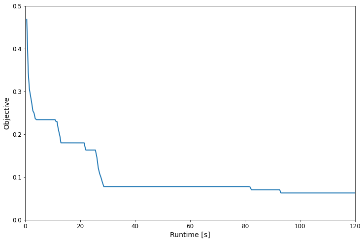
Analysing the results
The training history is stored in the results_df, the main fields
are the runtime and 'best' (the objective).
Note: You will get slightly different curves for different pairs of
scheduler/searcher, the time_out here is a bit too short to really
see the difference in a significant way (it would be better to set it to
>1000s). Generally speaking though, hyperband stopping / promotion +
model will tend to significantly outperform other combinations given
enough time.
results_df.head()
| bracket | elapsed_time | epoch | error | eval_time | objective | runtime | searcher_data_size | searcher_params_kernel_covariance_scale | searcher_params_kernel_inv_bw0 | ... | searcher_params_kernel_inv_bw7 | searcher_params_kernel_inv_bw8 | searcher_params_mean_mean_value | searcher_params_noise_variance | target_epoch | task_id | time_since_start | time_step | time_this_iter | best | |
|---|---|---|---|---|---|---|---|---|---|---|---|---|---|---|---|---|---|---|---|---|---|
| 0 | 0 | 0.485920 | 1 | 0.468750 | 0.481122 | 0.531250 | 0.574134 | NaN | 1.0 | 1.0 | ... | 1.0 | 1.0 | 0.0 | 0.001 | 9 | 0 | 0.576383 | 1.603414e+09 | 0.516324 | 0.468750 |
| 1 | 0 | 1.032178 | 2 | 0.344753 | 0.541059 | 0.655247 | 1.120392 | 1.0 | 1.0 | 1.0 | ... | 1.0 | 1.0 | 0.0 | 0.001 | 9 | 0 | 1.121254 | 1.603414e+09 | 0.546239 | 0.344753 |
| 2 | 0 | 1.453690 | 3 | 0.305314 | 0.419545 | 0.694686 | 1.541903 | 1.0 | 1.0 | 1.0 | ... | 1.0 | 1.0 | 0.0 | 0.001 | 9 | 0 | 1.542823 | 1.603414e+09 | 0.421512 | 0.305314 |
| 3 | 0 | 1.874310 | 4 | 0.288937 | 0.417926 | 0.711063 | 1.962523 | 2.0 | 1.0 | 1.0 | ... | 1.0 | 1.0 | 0.0 | 0.001 | 9 | 0 | 1.964000 | 1.603414e+09 | 0.420619 | 0.288937 |
| 4 | 0 | 2.298020 | 5 | 0.273061 | 0.421216 | 0.726939 | 2.386234 | 2.0 | 1.0 | 1.0 | ... | 1.0 | 1.0 | 0.0 | 0.001 | 9 | 0 | 2.386983 | 1.603414e+09 | 0.423711 | 0.273061 |
5 rows × 26 columns
import matplotlib.pyplot as plt

plt.figure(figsize=(12, 8))

runtime = results_df['runtime'].values
objective = results_df['best'].values

plt.plot(runtime, objective, lw=2)
plt.xticks(fontsize=12)
plt.xlim(0, 120)
plt.ylim(0, 0.5)
plt.yticks(fontsize=12)
plt.xlabel("Runtime [s]", fontsize=14)
plt.ylabel("Objective", fontsize=14)
Text(0, 0.5, 'Objective')
Diving Deeper
Now, you are ready to try HPO on your own machine learning models (if you use PyTorch, have a look at MNIST Training in PyTorch). While AutoGluon comes with well-chosen defaults, it can pay off to tune it to your specific needs. Here are some tips which may come useful.
Logging the Search Progress
First, it is a good idea in general to switch on debug_log, which
outputs useful information about the search progress. This is already
done in the example above.
The outputs show which configurations are chosen, stopped, or promoted.
For BO and BOHB, a range of information is displayed for every
get_config decision. This log output is very useful in order to
figure out what is going on during the search.
Configuring HyperbandScheduler
The most important knobs to turn with HyperbandScheduler are
max_t, grace_period, reduction_factor, brackets, and
type. The first three determine the rung levels at which stopping or
promotion decisions are being made.
The maximum resource level
max_t(usually, resource equates to epochs, somax_tis the maximum number of training epochs) is typically hardcoded intrain_fnpassed to the scheduler (this isrun_mlp_openmlin the example above). As already noted above, the value is best fixed in theag.argsdecorator asepochs=XYZ, it can then be accessed asargs.epochsin thetrain_fncode. If this is done, you do not have to passmax_twhen creating the scheduler.grace_periodandreduction_factordetermine the rung levels, which aregrace_period,grace_period * reduction_factor,grace_period * (reduction_factor ** 2), etc. All rung levels must be less or equal thanmax_t. It is recommended to makemax_tequal to the largest rung level. For example, ifgrace_period = 1,reduction_factor = 3, it is in general recommended to usemax_t = 9,max_t = 27, ormax_t = 81. Choosing amax_tvalue “off the grid” works against the successive halving principle that the total resources spent in a rung should be roughly equal between rungs. If in the example above, you setmax_t = 10, about a third of configurations reaching 9 epochs are allowed to proceed, but only for one more epoch.With
reduction_factor, you tune the extent to which successive halving filtering is applied. The larger this integer, the fewer configurations make it to higher number of epochs. Values 2, 3, 4 are commonly used.Finally,
grace_periodshould be set to the smallest resource (number of epochs) for which you expect any meaningful differentiation between configurations. Whilegrace_period = 1should always be explored, it may be too low for any meaningful stopping decisions to be made at the first rung.bracketssets the maximum number of brackets in Hyperband (make sure to study the Hyperband paper or follow-ups for details). Forbrackets = 1, you are running successive halving (single bracket). Higher brackets have larger effectivegrace_periodvalues (so runs are not stopped until later), yet are also chosen with less probability. We recommend to always consider successive halving (brackets = 1) in a comparison.Finally, with
type(valuesstopping,promotion) you are choosing different ways of extending successive halving scheduling to the asynchronous case. The method for the defaultstoppingis simpler and seems to perform well, butpromotionis more careful promoting configurations to higher resource levels, which can work better in some cases.
Asynchronous BOHB
Finally, here are some ideas for tuning asynchronous BOHB, apart from
tuning its HyperbandScheduling component. You need to pass these
options in search_options.
We support a range of different surrogate models over the criterion functions across resource levels. All of them are jointly dependent Gaussian process models, meaning that data collected at all resource levels are modelled together. The surrogate model is selected by
gp_resource_kernel, values arematern52,matern52-res-warp,exp-decay-sum,exp-decay-combined,exp-decay-delta1. These are variants of either a joint Matern 5/2 kernel over configuration and resource, or the exponential decay model. Details about the latter can be found here.Fitting a Gaussian process surrogate model to data encurs a cost which scales cubically with the number of datapoints. When applied to expensive deep learning workloads, even multi-fidelity asynchronous BOHB is rarely running up more than 100 observations or so (across all rung levels and brackets), and the GP computations are subdominant. However, if you apply it to cheaper
train_fnand find yourself beyond 2000 total evaluations, the cost of GP fitting can become painful. In such a situation, you can explore the optionsopt_skip_periodandopt_skip_num_max_resource. The basic idea is as follows. By far the most expensive part of aget_configcall (picking the next configuration) is the refitting of the GP model to past data (this entails re-optimizing hyperparameters of the surrogate model itself). The options allow you to skip this expensive step for mostget_configcalls, after some initial period. Check the docstrings for details about these options. If you find yourself in such a situation and gain experience with these skipping features, make sure to contact the AutoGluon developers – we would love to learn about your use case.