Image Classification - Search Space and Hyperparameter Optimization (HPO)¶

While the Image Classification - Quick Start introduced basic usage of AutoGluon fit, evaluate, predict with default configurations, this tutorial dives into the various options that you can specify for more advanced control over the fitting process.

These options include: - Defining the search space of various hyperparameter values for the training of neural networks - Specifying how to search through your choosen hyperparameter space - Specifying how to schedule jobs to train a network under a particular hyperparameter configuration.

The advanced functionalities of AutoGluon enable you to use your external knowledge about your particular prediction problem and computing resources to guide the training process. If properly used, you may be able to achieve superior performance within less training time.

Tip: If you are new to AutoGluon, review Image Classification - Quick Start to learn the basics of the AutoGluon API.

We begin by letting AutoGluon know that ImageClassification is the task of interest:

import autogluon.core as ag
from autogluon.vision import ImageClassification as task

Create AutoGluon Dataset¶

Let’s first create the dataset using the same subset of the Shopee-IET dataset as the Image Classification - Quick Start tutorial. Recall that because we only specify the train_path, a 90/10 train/validation split is automatically performed.

filename = ag.download('https://autogluon.s3.amazonaws.com/datasets/shopee-iet.zip')
ag.unzip(filename)

'data'

dataset = task.Dataset('data/train')

Specify which Networks to Try¶

We start with specifying the pretrained neural network candidates. Given such a list, AutoGluon tries to train different networks from this list to identify the best-performing candidate. This is an example of a autogluon.core.space.Categorical search space, in which there are a limited number of values to choose from.

import gluoncv as gcv

@ag.func(
    multiplier=ag.Categorical(0.25, 0.5),
)
def get_mobilenet(multiplier):
    return gcv.model_zoo.MobileNetV2(multiplier=multiplier, classes=4)

net = ag.space.Categorical('mobilenet0.25', get_mobilenet())
print(net)

Categorical['mobilenet0.25', AutoGluonObject]

Specify the Optimizer and Its Search Space¶

Similarly, we can manually specify the optimizer candidates. We can construct another search space to identify which optimizer works best for our task, and also identify the best hyperparameter configurations for this optimizer. Additionally, we can customize the optimizer-specific hyperparameters search spaces, such as learning rate and weight decay using autogluon.core.space.Real.

from mxnet import optimizer as optim

@ag.obj(
    learning_rate=ag.space.Real(1e-4, 1e-2, log=True),
    momentum=ag.space.Real(0.85, 0.95),
    wd=ag.space.Real(1e-6, 1e-2, log=True)
)
class NAG(optim.NAG):
    pass

optimizer = NAG()
print(optimizer)

AutoGluonObject -- NAG

Search Algorithms¶

In AutoGluon, autogluon.core.searcher supports different search search strategies for both hyperparameter optimization and architecture search. Beyond simply specifying the space of hyperparameter configurations to search over, you can also tell AutoGluon what strategy it should employ to actually search through this space. This process of finding good hyperparameters from a given search space is commonly referred to as hyperparameter optimization (HPO) or hyperparameter tuning. autogluon.core.scheduler orchestrates how individual training jobs are scheduled. We currently support FIFO (standard) and Hyperband scheduling, along with search by random sampling or Bayesian optimization. These basic techniques are rendered surprisingly powerful by AutoGluon’s support of asynchronous parallel execution.

Bayesian Optimization¶

Here is an example of using Bayesian Optimization using autogluon.core.searcher.GPFIFOSearcher.

Bayesian Optimization fits a probabilistic surrogate model to estimate the function that relates each hyperparameter configuration to the resulting performance of a model trained under this hyperparameter configuration. Our implementation makes use of a Gaussian process surrogate model along with expected improvement as acquisition function. It has been developed specifically to support asynchronous parallel evaluations.

time_limits = 2*60
epochs = 2

classifier = task.fit(dataset,
                      net=net,
                      optimizer=optimizer,
                      search_strategy='bayesopt',
                      time_limits=time_limits,
                      epochs=epochs,
                      ngpus_per_trial=1,
                      num_trials=2)

print('Top-1 val acc: %.3f' % classifier.results[classifier.results['reward_attr']])

scheduler: FIFOScheduler(
DistributedResourceManager{
(Remote: Remote REMOTE_ID: 0,
    <Remote: 'inproc://172.31.38.222/18200/1' processes=1 threads=8, memory=33.24 GB>, Resource: NodeResourceManager(8 CPUs, 1 GPUs))
})

HBox(children=(HTML(value=''), FloatProgress(value=0.0, max=2.0), HTML(value='')))

[Epoch 2] Validation: 0.412: 100%|██████████| 2/2 [00:09<00:00,  5.00s/it]

[Epoch 2] Validation: 0.312: 100%|██████████| 2/2 [00:09<00:00,  4.92s/it]
[Epoch 2] training: accuracy=0.357: 100%|██████████| 2/2 [00:09<00:00,  4.81s/it]

Top-1 val acc: 0.412

The BO searcher can be configured by search_options, see autogluon.core.searcher.GPFIFOSearcher. Load the test dataset and evaluate:

test_dataset = task.Dataset('data/test', train=False)

test_acc = classifier.evaluate(test_dataset)
print('Top-1 test acc: %.3f' % test_acc)

accuracy: 0.296875: 100%|██████████| 1/1 [00:00<00:00,  2.65it/s]

Top-1 test acc: 0.297

Note that num_trials=2 above is only used to speed up the tutorial. In normal practice, it is common to only use time_limits and drop num_trials.

Hyperband Early Stopping¶

AutoGluon currently supports scheduling trials in serial order and with early stopping (e.g., if the performance of the model early within training already looks bad, the trial may be terminated early to free up resources). Here is an example of using an early stopping scheduler autogluon.core.scheduler.HyperbandScheduler. scheduler_options is used to configure the scheduler. In this example, we run Hyperband with a single bracket, and stop/go decisions are made after 1 and 2 epochs (grace_period, grace_period * reduction_factor):

scheduler_options = {
    'grace_period': 1,
    'reduction_factor': 2,
    'brackets': 1}

classifier = task.fit(dataset,
                      net=net,
                      optimizer=optimizer,
                      search_strategy='hyperband',
                      epochs=4,
                      num_trials=2,
                      verbose=False,
                      plot_results=True,
                      ngpus_per_trial=1,
                      scheduler_options=scheduler_options)

print('Top-1 val acc: %.3f' % classifier.results[classifier.results['reward_attr']])

scheduler: HyperbandScheduler(terminator: HyperbandBracketManager(reward_attr: classification_reward, time_attr: epoch, rung_levels: [1, 2, 4], max_t: 4, rung_systems: [Rung system: Iter 4.000: None | Iter 2.000: None | Iter 1.000: None])

HBox(children=(HTML(value=''), FloatProgress(value=0.0, max=2.0), HTML(value='')))

[Epoch 4] training: accuracy=0.586:  75%|███████▌  | 3/4 [00:19<00:06,  6.48s/it]

[Epoch 1] training: accuracy=0.269:   0%|          | 0/4 [00:10<?, ?it/s]
[Epoch 4] training: accuracy=0.510: 100%|██████████| 4/4 [00:19<00:00,  4.83s/it]

../../_images/output_hpo_19f8b4_14_5.png

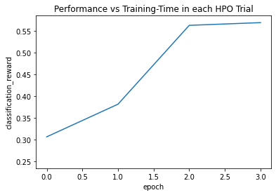
Top-1 val acc: 0.569

The test top-1 accuracy are:

test_acc = classifier.evaluate(test_dataset)
print('Top-1 test acc: %.3f' % test_acc)

accuracy: 0.671875: 100%|██████████| 1/1 [00:00<00:00,  3.04it/s]

Top-1 test acc: 0.672

Bayesian Optimization and Hyperband¶

While Hyperband scheduling is normally driven by a random searcher, AutoGluon also provides Hyperband together with Bayesian optimization. The tuning of expensive DL models typically works best with this combination.

scheduler_options = {
    'grace_period': 1,
    'reduction_factor': 2,
    'brackets': 1}

classifier = task.fit(dataset,
                      net=net,
                      optimizer=optimizer,
                      search_strategy='bayesopt_hyperband',
                      epochs=4,
                      num_trials=2,
                      verbose=False,
                      plot_results=True,
                      ngpus_per_trial=1,
                      scheduler_options=scheduler_options)

print('Top-1 val acc: %.3f' % classifier.results[classifier.results['reward_attr']])

scheduler: HyperbandScheduler(terminator: HyperbandBracketManager(reward_attr: classification_reward, time_attr: epoch, rung_levels: [1, 2, 4], max_t: 4, rung_systems: [Rung system: Iter 4.000: None | Iter 2.000: None | Iter 1.000: None])

HBox(children=(HTML(value=''), FloatProgress(value=0.0, max=2.0), HTML(value='')))

[Epoch 4] training: accuracy=0.566:  75%|███████▌  | 3/4 [00:19<00:06,  6.45s/it]

[Epoch 1] training: accuracy=0.356:   0%|          | 0/4 [00:04<?, ?it/s]
[Epoch 4] training: accuracy=0.496: 100%|██████████| 4/4 [00:19<00:00,  4.79s/it]

../../_images/output_hpo_19f8b4_18_5.png

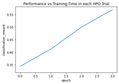
Top-1 val acc: 0.569

The test top-1 accuracy are:

test_acc = classifier.evaluate(test_dataset)
print('Top-1 test acc: %.3f' % test_acc)

accuracy: 0.65625: 100%|██████████| 1/1 [00:00<00:00,  3.15it/s]

Top-1 test acc: 0.656

For a comparison of different search algorithms and scheduling strategies, see Search Algorithms. For more options using fit, see autogluon.vision.ImageClassification.