Forecasting Time Series - Quick Start

Via a simple fit() call, AutoGluon can train and tune

• simple forecasting models (e.g., ARIMA, ETS, Theta),

• powerful deep learning models (e.g., DeepAR, Temporal Fusion Transformer),

• tree-based models (e.g., XGBoost, CatBoost, LightGBM),

• an ensemble that combines predictions of other models

to produce multi-step ahead probabilistic forecasts for univariate time series data.

This tutorial demonstrates how to quickly start using AutoGluon to generate hourly forecasts for the M4 forecasting competition dataset.

Loading time series data as a TimeSeriesDataFrame

First, we import some required modules

import pandas as pd
from autogluon.timeseries import TimeSeriesDataFrame, TimeSeriesPredictor

To use autogluon.timeseries, we will only need the following two classes:

• TimeSeriesDataFrame stores a dataset consisting of multiple time series.

• TimeSeriesPredictor takes care of fitting, tuning and selecting the best forecasting models, as well as generating new forecasts.

We load a subset of the M4 hourly dataset as a pandas.DataFrame

df = pd.read_csv("https://autogluon.s3.amazonaws.com/datasets/timeseries/m4_hourly_subset/train.csv")
df.head()

	item_id	timestamp	target
0	H1	1750-01-01 00:00:00	605.0
1	H1	1750-01-01 01:00:00	586.0
2	H1	1750-01-01 02:00:00	586.0
3	H1	1750-01-01 03:00:00	559.0
4	H1	1750-01-01 04:00:00	511.0

AutoGluon expects time series data in long format. Each row of the data frame contains a single observation (timestep) of a single time series represented by

• unique ID of the time series ("item_id") as int or str

• timestamp of the observation ("timestamp") as a pandas.Timestamp or compatible format

• numeric value of the time series ("target")

The raw dataset should always follow this format with at least three columns for unique ID, timestamp, and target value, but the names of these columns can be arbitrary. It is important, however, that we provide the names of the columns when constructing a TimeSeriesDataFrame that is used by AutoGluon. AutoGluon will raise an exception if the data doesn’t match the expected format.

train_data = TimeSeriesDataFrame.from_data_frame(
    df,
    id_column="item_id",
    timestamp_column="timestamp"
)
train_data.head()

		target
item_id	timestamp
H1	1750-01-01 00:00:00	605.0
	1750-01-01 01:00:00	586.0
	1750-01-01 02:00:00	586.0
	1750-01-01 03:00:00	559.0
	1750-01-01 04:00:00	511.0

We refer to each individual time series stored in a TimeSeriesDataFrame as an item. For example, items might correspond to different products in demand forecasting, or to different stocks in financial datasets. This setting is also referred to as a panel of time series. Note that this is not the same as multivariate forecasting — AutoGluon generates forecasts for each time series individually, without modeling interactions between different items (time series).

TimeSeriesDataFrame inherits from pandas.DataFrame, so all attributes and methods of pandas.DataFrame are available in a TimeSeriesDataFrame. It also provides other utility functions, such as loaders for different data formats (see autogluon.timeseries.TimeSeriesDataFrame for details).

Training time series models with TimeSeriesPredictor.fit

To forecast future values of the time series, we need to create a TimeSeriesPredictor object.

Models in autogluon.timeseries forecast time series multiple steps into the future. We choose the number of these steps — the prediction length (also known as the forecast horizon) — depending on our task. For example, our dataset contains time series measured at hourly frequency, so we set prediction_length = 48 to train models that forecast up to 48 hours into the future.

We instruct AutoGluon to save trained models in the folder ./autogluon-m4-hourly. We also specify that AutoGluon should rank models according to symmetric mean absolute percentage error (sMAPE), and that data that we want to forecast is stored in the column "target" of the TimeSeriesDataFrame.

predictor = TimeSeriesPredictor(
    prediction_length=48,
    path="autogluon-m4-hourly",
    target="target",
    eval_metric="sMAPE",
)

predictor.fit(
    train_data,
    presets="medium_quality",
    time_limit=600,
)

================ TimeSeriesPredictor ================
TimeSeriesPredictor.fit() called
Setting presets to: medium_quality
Fitting with arguments:
{'enable_ensemble': True,
 'evaluation_metric': 'sMAPE',
 'hyperparameter_tune_kwargs': None,
 'hyperparameters': 'medium_quality',
 'prediction_length': 48,
 'random_seed': None,
 'target': 'target',
 'time_limit': 600}
Provided training data set with 148060 rows, 200 items (item = single time series). Average time series length is 740.3.
Training artifacts will be saved to: /home/ci/autogluon/docs/_build/eval/tutorials/timeseries/autogluon-m4-hourly
=====================================================
AutoGluon will save models to autogluon-m4-hourly/
AutoGluon will gauge predictive performance using evaluation metric: 'sMAPE'
    This metric's sign has been flipped to adhere to being 'higher is better'. The reported score can be multiplied by -1 to get the metric value.

Provided dataset contains following columns:
    target:           'target'
tuning_data is None. Will use the last prediction_length = 48 time steps of each time series as a hold-out validation set.

Starting training. Start time is 2023-03-04 20:39:58
Models that will be trained: ['Naive', 'SeasonalNaive', 'ETS', 'Theta', 'ARIMA', 'AutoETS', 'AutoGluonTabular', 'DeepAR']
Training timeseries model Naive. Training for up to 599.89s of the 599.89s of remaining time.
    -0.4341       = Validation score (-sMAPE)
    0.60    s     = Training runtime
    4.56    s     = Validation (prediction) runtime
Training timeseries model SeasonalNaive. Training for up to 594.72s of the 594.72s of remaining time.
    -0.1686       = Validation score (-sMAPE)
    0.60    s     = Training runtime
    0.40    s     = Validation (prediction) runtime
Training timeseries model ETS. Training for up to 593.70s of the 593.70s of remaining time.
    -0.2666       = Validation score (-sMAPE)
    0.60    s     = Training runtime
    34.50   s     = Validation (prediction) runtime
Training timeseries model Theta. Training for up to 558.60s of the 558.60s of remaining time.
    -0.2236       = Validation score (-sMAPE)
    0.60    s     = Training runtime
    12.23   s     = Validation (prediction) runtime
Training timeseries model ARIMA. Training for up to 545.75s of the 545.75s of remaining time.
    -0.5269       = Validation score (-sMAPE)
    0.60    s     = Training runtime
    14.27   s     = Validation (prediction) runtime
Training timeseries model AutoETS. Training for up to 530.87s of the 530.87s of remaining time.
    -0.2381       = Validation score (-sMAPE)
    0.60    s     = Training runtime
    121.90  s     = Validation (prediction) runtime
Training timeseries model AutoGluonTabular. Training for up to 408.37s of the 408.37s of remaining time.
    -0.1089       = Validation score (-sMAPE)
    45.21   s     = Training runtime
    0.76    s     = Validation (prediction) runtime
Training timeseries model DeepAR. Training for up to 362.40s of the 362.40s of remaining time.
    -0.1481       = Validation score (-sMAPE)
    95.30   s     = Training runtime
    2.20    s     = Validation (prediction) runtime
Fitting simple weighted ensemble.
    -0.1079       = Validation score (-sMAPE)
    7.70    s     = Training runtime
    7.52    s     = Validation (prediction) runtime
Training complete. Models trained: ['Naive', 'SeasonalNaive', 'ETS', 'Theta', 'ARIMA', 'AutoETS', 'AutoGluonTabular', 'DeepAR', 'WeightedEnsemble']
Total runtime: 346.26 s
Best model: WeightedEnsemble
Best model score: -0.1079

<autogluon.timeseries.predictor.TimeSeriesPredictor at 0x7f3fd6c251f0>

Here we used the "medium_quality" presets and limited the training time to 10 minutes (600 seconds). The presets define which models AutoGluon will try to fit. For medium_quality presets, these are simple baselines (Naive, SeasonalNaive), statistical models (ARIMA, ETS, Theta), tree-based models XGBoost, LightGBM and CatBoost wrapped by AutoGluonTabular, a deep learning model DeepAR, and a weighted ensemble combining these. Other available presets for TimeSeriesPredictor are "fast_training", "high_quality" and "best_quality". Higher quality presets will usually produce more accurate forecasts but take longer to train and may produce less computationally efficient models.

Inside fit(), AutoGluon will train as many models as possible within the given time limit. Trained models are then ranked based on their performance on an internal validation set. By default, this validation set is constructed by holding out the last prediction_length timesteps of each time series in train_data.

Generating forecasts with TimeSeriesPredictor.predict

We can now use the fitted TimeSeriesPredictor to forecast the future time series values. By default, AutoGluon will make forecasts using the model that had the best score on the internal validation set. The forecast always includes predictions for the next prediction_length timesteps, starting from the end of each time series in train_data.

predictions = predictor.predict(train_data)
predictions.head()

Global seed set to 123
Model not specified in predict, will default to the model with the best validation score: WeightedEnsemble

		mean	0.1	0.2	0.3	0.4	0.5	0.6	0.7	0.8	0.9
item_id	timestamp
H1	1750-01-30 04:00:00	657.185721	584.988170	620.348103	638.282653	649.226638	657.508168	665.209871	674.435057	688.809049	721.791643
	1750-01-30 05:00:00	587.819460	515.392420	550.901686	568.885141	579.884646	588.139793	595.860552	605.148147	619.627062	652.847356
	1750-01-30 06:00:00	551.021436	478.029042	513.521607	531.736358	542.798419	551.329943	559.175235	568.599921	583.261533	616.574716
	1750-01-30 07:00:00	514.061223	440.751066	476.342580	494.628764	505.883682	514.294612	522.338167	531.829933	546.419694	580.151047
	1750-01-30 08:00:00	488.126182	414.369102	449.988927	468.277394	479.621589	488.228078	496.213210	505.951036	520.728707	554.703486

AutoGluon produces a probabilistic forecast: in addition to predicting the mean (expected value) of the time series in the future, models also provide the quantiles of the forecast distribution. The quantile forecasts give us an idea about the range of possible outcomes. For example, if the "0.1" quantile is equal to 500.0, it means that the model predicts a 10% chance that the target value will be below 500.0.

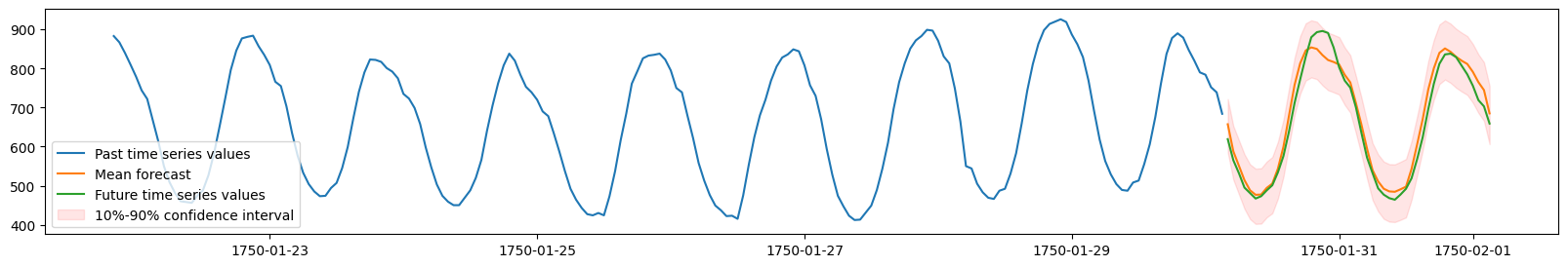
We will now visualize the forecast and the actually observed values for one of the time series in the dataset. We plot the mean forecast, as well as the 10% and 90% quantiles to show the range of potential outcomes.

import matplotlib.pyplot as plt

# TimeSeriesDataFrame can also be loaded directly from a file
test_data = TimeSeriesDataFrame.from_path("https://autogluon.s3.amazonaws.com/datasets/timeseries/m4_hourly_subset/test.csv")

plt.figure(figsize=(20, 3))

item_id = "H1"
y_past = train_data.loc[item_id]["target"]
y_pred = predictions.loc[item_id]
y_test = test_data.loc[item_id]["target"][-48:]

plt.plot(y_past[-200:], label="Past time series values")
plt.plot(y_pred["mean"], label="Mean forecast")
plt.plot(y_test, label="Future time series values")

plt.fill_between(
    y_pred.index, y_pred["0.1"], y_pred["0.9"], color="red", alpha=0.1, label=f"10%-90% confidence interval"
)
plt.legend();

Loaded data from: https://autogluon.s3.amazonaws.com/datasets/timeseries/m4_hourly_subset/test.csv | Columns = 3 / 3 | Rows = 157660 -> 157660

Evaluating the performance of different models

We can view the performance of each model AutoGluon has trained via the leaderboard() method. We provide the test data set to the leaderboard function to see how well our fitted models are doing on the unseen test data. The leaderboard also includes the validation scores computed on the internal validation dataset.

In AutoGluon leaderboards, higher scores always correspond to better predictive performance. Therefore our sMAPE scores are multiplied by -1, such that higher “negative sMAPE”s correspond to more accurate forecasts.

# The test score is computed using the last
# prediction_length=48 timesteps of each time series in test_data
predictor.leaderboard(test_data, silent=True)

Additional data provided, testing on additional data. Resulting leaderboard will be sorted according to test score (score_test).

	model	score_test	score_val	pred_time_test	pred_time_val	fit_time_marginal	fit_order
0	WeightedEnsemble	-0.103177	-0.107912	3.098925	7.518984	7.696324	9
1	AutoGluonTabular	-0.105318	-0.108919	2.155357	0.760451	45.206022	7
2	SeasonalNaive	-0.119063	-0.168566	4.653306	0.399796	0.602032	2
3	DeepAR	-0.139270	-0.148051	2.241937	2.200583	95.301887	8
4	Theta	-0.194352	-0.223630	13.234833	12.233251	0.601030	4
5	AutoETS	-0.195432	-0.238137	127.289864	121.899619	0.598926	6
6	ETS	-0.218012	-0.266572	35.668317	34.495035	0.600495	3
7	Naive	-0.453291	-0.434068	0.182284	4.557950	0.598527	1
8	ARIMA	-0.518139	-0.526885	15.346318	14.268253	0.596856	5

Summary

We used autogluon.timeseries to make probabilistic multi-step forecasts on the M4 Hourly dataset. Check out Forecasting Time Series - In Depth to learn about the advanced capabilities of AutoGluon for time series forecasting.