Text Prediction - Quick Start

Here we briefly demonstrate the TextPredictor, which helps you automatically train and deploy models for various Natural Language Processing (NLP) tasks. This tutorial presents two examples of NLP tasks:

• Sentiment Analysis

• Sentence Similarity

The general usage of the TextPredictor is similar to AutoGluon’s TabularPredictor. We format NLP datasets as tables where certain columns contain text fields and a special column contains the labels to predict, and each row corresponds to one training example. Here, the labels can be discrete categories (classification) or numerical values (regression).

%matplotlib inline

import numpy as np
import warnings
import matplotlib.pyplot as plt
warnings.filterwarnings('ignore')
np.random.seed(123)

Sentiment Analysis Task

First, we consider the Stanford Sentiment Treebank (SST) dataset, which consists of movie reviews and their associated sentiment. Given a new movie review, the goal is to predict the sentiment reflected in the text (in this case a binary classification, where reviews are labeled as 1 if they convey a positive opinion and labeled as 0 otherwise). Let’s first load and look at the data, noting the labels are stored in a column called label.

from autogluon.core import TabularDataset
train_data = TabularDataset('https://autogluon-text.s3-accelerate.amazonaws.com/glue/sst/train.parquet')
test_data = TabularDataset('https://autogluon-text.s3-accelerate.amazonaws.com/glue/sst/dev.parquet')
subsample_size = 1000  # subsample data for faster demo, try setting this to larger values
train_data = train_data.sample(n=subsample_size, random_state=0)
train_data.head(10)

	sentence	label
43787	very pleasing at its best moments	1
16159	, american chai is enough to make you put away...	0
59015	too much like an infomercial for ram dass 's l...	0
5108	a stirring visual sequence	1
67052	cool visual backmasking	1
35938	hard ground	0
49879	the striking , quietly vulnerable personality ...	1
51591	pan nalin 's exposition is beautiful and myste...	1
56780	wonderfully loopy	1
28518	most beautiful , evocative	1

Above the data happen to be stored in a Parquet table format, but you can also directly load() data from a CSV file instead. While here we load files from AWS S3 cloud storage, these could instead be local files on your machine. After loading, train_data is simply a Pandas DataFrame, where each row represents a different training example (for machine learning to be appropriate, the rows should be independent and identically distributed).

Training

To ensure this tutorial runs quickly, we simply call fit() with a subset of 1000 training examples and limit its runtime to approximately 1 minute. To achieve reasonable performance in your applications, you are recommended to set much longer time_limit (eg. 1 hour), or do not specify time_limit at all (time_limit=None).

from autogluon.text import TextPredictor

predictor = TextPredictor(label='label', eval_metric='acc', path='./ag_sst')
predictor.fit(train_data, time_limit=60)

Global seed set to 123
Warning: path already exists! This predictor may overwrite an existing predictor! path="./ag_sst/"
Using 16bit native Automatic Mixed Precision (AMP)
Trainer already configured with model summary callbacks: [<class 'pytorch_lightning.callbacks.model_summary.ModelSummary'>]. Skipping setting a default ModelSummary callback.
GPU available: True, used: True
TPU available: False, using: 0 TPU cores
IPU available: False, using: 0 IPUs
LOCAL_RANK: 0 - CUDA_VISIBLE_DEVICES: [0]

  | Name              | Type                         | Params
-------------------------------------------------------------------
0 | model             | HFAutoModelForTextPrediction | 108 M
1 | validation_metric | Accuracy                     | 0
2 | loss_func         | CrossEntropyLoss             | 0
-------------------------------------------------------------------
108 M     Trainable params
0         Non-trainable params
108 M     Total params
217.786   Total estimated model params size (MB)

Validation sanity check: 0it [00:00, ?it/s]

Global seed set to 123

Training: 0it [00:00, ?it/s]

Validating: 0it [00:00, ?it/s]

Epoch 0, global step 3: val_acc reached 0.59000 (best 0.59000), saving model to "/var/lib/jenkins/workspace/workspace/autogluon-tutorial-text-v3/docs/_build/eval/tutorials/text_prediction/ag_sst/epoch=0-step=3.ckpt" as top 3

Validating: 0it [00:00, ?it/s]

Epoch 0, global step 6: val_acc reached 0.65500 (best 0.65500), saving model to "/var/lib/jenkins/workspace/workspace/autogluon-tutorial-text-v3/docs/_build/eval/tutorials/text_prediction/ag_sst/epoch=0-step=6.ckpt" as top 3

Validating: 0it [00:00, ?it/s]

Epoch 1, global step 10: val_acc reached 0.66000 (best 0.66000), saving model to "/var/lib/jenkins/workspace/workspace/autogluon-tutorial-text-v3/docs/_build/eval/tutorials/text_prediction/ag_sst/epoch=1-step=10.ckpt" as top 3

Validating: 0it [00:00, ?it/s]

Epoch 1, global step 13: val_acc reached 0.73000 (best 0.73000), saving model to "/var/lib/jenkins/workspace/workspace/autogluon-tutorial-text-v3/docs/_build/eval/tutorials/text_prediction/ag_sst/epoch=1-step=13.ckpt" as top 3

Validating: 0it [00:00, ?it/s]

Epoch 2, global step 17: val_acc reached 0.80500 (best 0.80500), saving model to "/var/lib/jenkins/workspace/workspace/autogluon-tutorial-text-v3/docs/_build/eval/tutorials/text_prediction/ag_sst/epoch=2-step=17.ckpt" as top 3

Validating: 0it [00:00, ?it/s]

Epoch 2, global step 20: val_acc reached 0.85000 (best 0.85000), saving model to "/var/lib/jenkins/workspace/workspace/autogluon-tutorial-text-v3/docs/_build/eval/tutorials/text_prediction/ag_sst/epoch=2-step=20.ckpt" as top 3
Time limit reached. Elapsed time is 0:01:05. Signaling Trainer to stop.

Validating: 0it [00:00, ?it/s]

Epoch 3, global step 21: val_acc reached 0.85000 (best 0.85000), saving model to "/var/lib/jenkins/workspace/workspace/autogluon-tutorial-text-v3/docs/_build/eval/tutorials/text_prediction/ag_sst/epoch=3-step=21.ckpt" as top 3

<autogluon.text.text_prediction.predictor.TextPredictor at 0x7f1b257cf3d0>

Above we specify that: the column named label contains the label values to predict, AutoGluon should optimize its predictions for the accuracy evaluation metric, trained models should be saved in the ag_sst folder, and training should run for around 60 seconds.

Evaluation

After training, we can easily evaluate our predictor on separate test data formatted similarly to our training data.

test_score = predictor.evaluate(test_data)
print(test_score)

Using 16bit native Automatic Mixed Precision (AMP)
GPU available: True, used: True
TPU available: False, using: 0 TPU cores
IPU available: False, using: 0 IPUs
LOCAL_RANK: 0 - CUDA_VISIBLE_DEVICES: [0]

Predicting: 0it [00:00, ?it/s]

{'acc': 0.8027522935779816}

By default, evaluate() will report the evaluation metric previously specified, which is accuracy in our example. You may also specify additional metrics, e.g. F1 score, when calling evaluate.

test_score = predictor.evaluate(test_data, metrics=['acc', 'f1'])
print(test_score)

Using 16bit native Automatic Mixed Precision (AMP)
GPU available: True, used: True
TPU available: False, using: 0 TPU cores
IPU available: False, using: 0 IPUs
LOCAL_RANK: 0 - CUDA_VISIBLE_DEVICES: [0]

Predicting: 0it [00:00, ?it/s]

{'acc': 0.8027522935779816, 'f1': 0.831041257367387}

Prediction

And you can easily obtain predictions from these models by calling predictor.predict().

sentence1 = "it's a charming and often affecting journey."
sentence2 = "It's slow, very, very, very slow."
predictions = predictor.predict({'sentence': [sentence1, sentence2]})
print('"Sentence":', sentence1, '"Predicted Sentiment":', predictions.iloc[0])
print('"Sentence":', sentence2, '"Predicted Sentiment":', predictions.iloc[1])

Using 16bit native Automatic Mixed Precision (AMP)
GPU available: True, used: True
TPU available: False, using: 0 TPU cores
IPU available: False, using: 0 IPUs
LOCAL_RANK: 0 - CUDA_VISIBLE_DEVICES: [0]

Predicting: 0it [00:00, ?it/s]

"Sentence": it's a charming and often affecting journey. "Predicted Sentiment": 1
"Sentence": It's slow, very, very, very slow. "Predicted Sentiment": 0

For classification tasks, you can ask for predicted class-probabilities instead of predicted classes.

probs = predictor.predict_proba({'sentence': [sentence1, sentence2]})
print('"Sentence":', sentence1, '"Predicted Class-Probabilities":', probs.iloc[0])
print('"Sentence":', sentence2, '"Predicted Class-Probabilities":', probs.iloc[1])

Using 16bit native Automatic Mixed Precision (AMP)
GPU available: True, used: True
TPU available: False, using: 0 TPU cores
IPU available: False, using: 0 IPUs
LOCAL_RANK: 0 - CUDA_VISIBLE_DEVICES: [0]

Predicting: 0it [00:00, ?it/s]

"Sentence": it's a charming and often affecting journey. "Predicted Class-Probabilities": 0    0.03475
1    0.96525
Name: 0, dtype: float32
"Sentence": It's slow, very, very, very slow. "Predicted Class-Probabilities": 0    0.713531
1    0.286469
Name: 1, dtype: float32

We can just as easily produce predictions over an entire dataset.

test_predictions = predictor.predict(test_data)
test_predictions.head()

Using 16bit native Automatic Mixed Precision (AMP)
GPU available: True, used: True
TPU available: False, using: 0 TPU cores
IPU available: False, using: 0 IPUs
LOCAL_RANK: 0 - CUDA_VISIBLE_DEVICES: [0]

Predicting: 0it [00:00, ?it/s]

0    1
1    1
2    1
3    1
4    0
Name: label, dtype: int64

Save and Load

The trained predictor is automatically saved at the end of fit(), and you can easily reload it.

loaded_predictor = TextPredictor.load('ag_sst')
loaded_predictor.predict_proba({'sentence': [sentence1, sentence2]})

Load pretrained checkpoint: ag_sst/model.ckpt
Using 16bit native Automatic Mixed Precision (AMP)
GPU available: True, used: True
TPU available: False, using: 0 TPU cores
IPU available: False, using: 0 IPUs
LOCAL_RANK: 0 - CUDA_VISIBLE_DEVICES: [0]

Predicting: 0it [00:00, ?it/s]

	0	1
0	0.034750	0.965250
1	0.713531	0.286469

You can also save the predictor to any location by calling .save().

loaded_predictor.save('my_saved_dir')
loaded_predictor2 = TextPredictor.load('my_saved_dir')
loaded_predictor2.predict_proba({'sentence': [sentence1, sentence2]})

Load pretrained checkpoint: my_saved_dir/model.ckpt
Using 16bit native Automatic Mixed Precision (AMP)
GPU available: True, used: True
TPU available: False, using: 0 TPU cores
IPU available: False, using: 0 IPUs
LOCAL_RANK: 0 - CUDA_VISIBLE_DEVICES: [0]

Predicting: 0it [00:00, ?it/s]

	0	1
0	0.034750	0.965250
1	0.713531	0.286469

Extract Embeddings

You can also use a trained predictor to extract embeddings that maps each row of the data table to an embedding vector extracted from intermediate neural network representations of the row.

embeddings = predictor.extract_embedding(test_data)
print(embeddings)

Using 16bit native Automatic Mixed Precision (AMP)
GPU available: True, used: True
TPU available: False, using: 0 TPU cores
IPU available: False, using: 0 IPUs
LOCAL_RANK: 0 - CUDA_VISIBLE_DEVICES: [0]

Predicting: 0it [00:00, ?it/s]

[[-0.07428363  0.2043701   0.23956704 ...  0.15007006  0.05809359
   0.57036537]
 [-0.66558814  0.13521251  0.3106878  ...  0.25094986  0.03894259
   0.0274822 ]
 [ 0.32139373  0.23424031  0.30713102 ... -0.09012198  0.04438552
   0.62386334]
 ...
 [ 0.18162525  0.3314941   0.35503426 ... -0.3362026   0.02671325
   0.41504022]
 [-0.25507736  0.09467821  0.08750397 ... -0.28553712 -0.08461647
   0.33479375]
 [ 0.12279123  0.16600318  0.32927352 ... -0.00218988 -0.20963569
   0.26129323]]

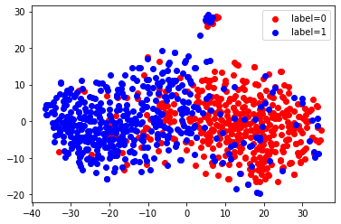
Here, we use TSNE to visualize these extracted embeddings. We can see that there are two clusters corresponding to our two labels, since this network has been trained to discriminate between these labels.

from sklearn.manifold import TSNE
X_embedded = TSNE(n_components=2, random_state=123).fit_transform(embeddings)
for val, color in [(0, 'red'), (1, 'blue')]:
    idx = (test_data['label'].to_numpy() == val).nonzero()
    plt.scatter(X_embedded[idx, 0], X_embedded[idx, 1], c=color, label=f'label={val}')
plt.legend(loc='best')

<matplotlib.legend.Legend at 0x7f1b4cb6f3a0>

Continuous Training

You can also load a predictor and call .fit() again to continue training the same predictor with new data.

new_predictor = TextPredictor.load('ag_sst')
new_predictor.fit(train_data, time_limit=30, save_path='ag_sst_continue_train')
test_score = new_predictor.evaluate(test_data, metrics=['acc', 'f1'])
print(test_score)

Load pretrained checkpoint: ag_sst/model.ckpt
Global seed set to 123
Using 16bit native Automatic Mixed Precision (AMP)
Trainer already configured with model summary callbacks: [<class 'pytorch_lightning.callbacks.model_summary.ModelSummary'>]. Skipping setting a default ModelSummary callback.
GPU available: True, used: True
TPU available: False, using: 0 TPU cores
IPU available: False, using: 0 IPUs
LOCAL_RANK: 0 - CUDA_VISIBLE_DEVICES: [0]

  | Name              | Type                         | Params
-------------------------------------------------------------------
0 | model             | HFAutoModelForTextPrediction | 108 M
1 | validation_metric | Accuracy                     | 0
2 | loss_func         | CrossEntropyLoss             | 0
-------------------------------------------------------------------
108 M     Trainable params
0         Non-trainable params
108 M     Total params
217.786   Total estimated model params size (MB)

Validation sanity check: 0it [00:00, ?it/s]

Global seed set to 123

Training: 0it [00:00, ?it/s]

Validating: 0it [00:00, ?it/s]

Epoch 0, global step 3: val_acc reached 0.88500 (best 0.88500), saving model to "/var/lib/jenkins/workspace/workspace/autogluon-tutorial-text-v3/docs/_build/eval/tutorials/text_prediction/ag_sst_continue_train/epoch=0-step=3.ckpt" as top 3

Validating: 0it [00:00, ?it/s]

Epoch 0, global step 6: val_acc reached 0.89500 (best 0.89500), saving model to "/var/lib/jenkins/workspace/workspace/autogluon-tutorial-text-v3/docs/_build/eval/tutorials/text_prediction/ag_sst_continue_train/epoch=0-step=6.ckpt" as top 3

Validating: 0it [00:00, ?it/s]

Epoch 1, global step 10: val_acc reached 0.92500 (best 0.92500), saving model to "/var/lib/jenkins/workspace/workspace/autogluon-tutorial-text-v3/docs/_build/eval/tutorials/text_prediction/ag_sst_continue_train/epoch=1-step=10.ckpt" as top 3
Time limit reached. Elapsed time is 0:00:32. Signaling Trainer to stop.

Validating: 0it [00:00, ?it/s]

Using 16bit native Automatic Mixed Precision (AMP)
GPU available: True, used: True
TPU available: False, using: 0 TPU cores
IPU available: False, using: 0 IPUs
LOCAL_RANK: 0 - CUDA_VISIBLE_DEVICES: [0]

Predicting: 0it [00:00, ?it/s]

{'acc': 0.875, 'f1': 0.8800880088008801}

Sentence Similarity Task

Next, let’s use AutoGluon to train a model for evaluating how semantically similar two sentences are. We use the Semantic Textual Similarity Benchmark dataset for illustration.

sts_train_data = TabularDataset('https://autogluon-text.s3-accelerate.amazonaws.com/glue/sts/train.parquet')[['sentence1', 'sentence2', 'score']]
sts_test_data = TabularDataset('https://autogluon-text.s3-accelerate.amazonaws.com/glue/sts/dev.parquet')[['sentence1', 'sentence2', 'score']]
sts_train_data.head(10)

	sentence1	sentence2	score
0	A plane is taking off.	An air plane is taking off.	5.00
1	A man is playing a large flute.	A man is playing a flute.	3.80
2	A man is spreading shreded cheese on a pizza.	A man is spreading shredded cheese on an uncoo...	3.80
3	Three men are playing chess.	Two men are playing chess.	2.60
4	A man is playing the cello.	A man seated is playing the cello.	4.25
5	Some men are fighting.	Two men are fighting.	4.25
6	A man is smoking.	A man is skating.	0.50
7	The man is playing the piano.	The man is playing the guitar.	1.60
8	A man is playing on a guitar and singing.	A woman is playing an acoustic guitar and sing...	2.20
9	A person is throwing a cat on to the ceiling.	A person throws a cat on the ceiling.	5.00

In this data, the column named score contains numerical values (which we’d like to predict) that are human-annotated similarity scores for each given pair of sentences.

print('Min score=', min(sts_train_data['score']), ', Max score=', max(sts_train_data['score']))

Min score= 0.0 , Max score= 5.0

Let’s train a regression model to predict these scores. Note that we only need to specify the label column and AutoGluon automatically determines the type of prediction problem and an appropriate loss function. Once again, you should increase the short time_limit below to obtain reasonable performance in your own applications.

predictor_sts = TextPredictor(label='score', path='./ag_sts')
predictor_sts.fit(sts_train_data, time_limit=60)

Global seed set to 123
Warning: path already exists! This predictor may overwrite an existing predictor! path="./ag_sts/"
Using 16bit native Automatic Mixed Precision (AMP)
Trainer already configured with model summary callbacks: [<class 'pytorch_lightning.callbacks.model_summary.ModelSummary'>]. Skipping setting a default ModelSummary callback.
GPU available: True, used: True
TPU available: False, using: 0 TPU cores
IPU available: False, using: 0 IPUs
LOCAL_RANK: 0 - CUDA_VISIBLE_DEVICES: [0]

  | Name              | Type                         | Params
-------------------------------------------------------------------
0 | model             | HFAutoModelForTextPrediction | 108 M
1 | validation_metric | MeanSquaredError             | 0
2 | loss_func         | MSELoss                      | 0
-------------------------------------------------------------------
108 M     Trainable params
0         Non-trainable params
108 M     Total params
217.785   Total estimated model params size (MB)

Validation sanity check: 0it [00:00, ?it/s]

Global seed set to 123

Training: 0it [00:00, ?it/s]

Validating: 0it [00:00, ?it/s]

Epoch 0, global step 20: val_rmse reached 0.59503 (best 0.59503), saving model to "/var/lib/jenkins/workspace/workspace/autogluon-tutorial-text-v3/docs/_build/eval/tutorials/text_prediction/ag_sts/epoch=0-step=20.ckpt" as top 3

Validating: 0it [00:00, ?it/s]

Epoch 0, global step 40: val_rmse reached 0.74501 (best 0.59503), saving model to "/var/lib/jenkins/workspace/workspace/autogluon-tutorial-text-v3/docs/_build/eval/tutorials/text_prediction/ag_sts/epoch=0-step=40.ckpt" as top 3
Time limit reached. Elapsed time is 0:01:00. Signaling Trainer to stop.

Validating: 0it [00:00, ?it/s]

Epoch 1, global step 60: val_rmse reached 0.46795 (best 0.46795), saving model to "/var/lib/jenkins/workspace/workspace/autogluon-tutorial-text-v3/docs/_build/eval/tutorials/text_prediction/ag_sts/epoch=1-step=60.ckpt" as top 3

<autogluon.text.text_prediction.predictor.TextPredictor at 0x7f1a7f3a4b80>

We again evaluate our trained model’s performance on separate test data. Below we choose to compute the following metrics: RMSE, Pearson Correlation, and Spearman Correlation.

test_score = predictor_sts.evaluate(sts_test_data, metrics=['rmse', 'pearsonr', 'spearmanr'])
print('RMSE = {:.2f}'.format(test_score['rmse']))
print('PEARSONR = {:.4f}'.format(test_score['pearsonr']))
print('SPEARMANR = {:.4f}'.format(test_score['spearmanr']))

Using 16bit native Automatic Mixed Precision (AMP)
GPU available: True, used: True
TPU available: False, using: 0 TPU cores
IPU available: False, using: 0 IPUs
LOCAL_RANK: 0 - CUDA_VISIBLE_DEVICES: [0]

Predicting: 0it [00:00, ?it/s]

RMSE = 0.74
PEARSONR = 0.8786
SPEARMANR = 0.8818

Let’s use our model to predict the similarity score between a few sentences.

sentences = ['The child is riding a horse.',
             'The young boy is riding a horse.',
             'The young man is riding a horse.',
             'The young man is riding a bicycle.']

score1 = predictor_sts.predict({'sentence1': [sentences[0]],
                                'sentence2': [sentences[1]]}, as_pandas=False)

score2 = predictor_sts.predict({'sentence1': [sentences[0]],
                                'sentence2': [sentences[2]]}, as_pandas=False)

score3 = predictor_sts.predict({'sentence1': [sentences[0]],
                                'sentence2': [sentences[3]]}, as_pandas=False)
print(score1, score2, score3)

Using 16bit native Automatic Mixed Precision (AMP)
GPU available: True, used: True
TPU available: False, using: 0 TPU cores
IPU available: False, using: 0 IPUs
LOCAL_RANK: 0 - CUDA_VISIBLE_DEVICES: [0]

Predicting: 0it [00:00, ?it/s]

Using 16bit native Automatic Mixed Precision (AMP)
GPU available: True, used: True
TPU available: False, using: 0 TPU cores
IPU available: False, using: 0 IPUs
LOCAL_RANK: 0 - CUDA_VISIBLE_DEVICES: [0]

Predicting: 0it [00:00, ?it/s]

Using 16bit native Automatic Mixed Precision (AMP)
GPU available: True, used: True
TPU available: False, using: 0 TPU cores
IPU available: False, using: 0 IPUs
LOCAL_RANK: 0 - CUDA_VISIBLE_DEVICES: [0]

Predicting: 0it [00:00, ?it/s]

4.3806043 3.034823 0.83805895

Although the TextPredictor is only designed for classification and regression tasks, it can directly be used for many NLP tasks if you properly format them into a data table. Note that there can be many text columns in this data table. Refer to the TextPredictor documentation to see all of the available methods/options.

Unlike TabularPredictor which trains/ensembles many different kinds of models,  TextPredictor fits only Transformer neural network models. These are fit to your data via transfer learning from pretrained NLP models like: BERT, ALBERT, and ELECTRA. TextPredictor also enables training on multi-modal data tables that contain text, numeric and categorical columns.

Note: TextPredictor uses pytorch as the default backend.